Reducing BigQuery Costs by 260x

In this blog post, we'll do a deep-dive into a simple trick that can reduce BigQuery costs by orders of magnitude. Specifically, we'll explore how clustering (similar to indexing in BigQuery world) large tables can significantly impact costs. We will walk through an example use-case for a common query pattern (MERGE), where clustering reduces the amount of data processed by BigQuery from 10GB to 37MB, resulting in a cost reduction of ~260X.
Setup
The setup involves a common Data Warehousing scenario of transforming raw data from multiple sources into a consumable format through the MERGE command. Now, let's delve into the data model:
There are two groups of tables, each containing two tables. One group of tables is clustered based on the
idcolumn, while the tables in the other group are not clustered.One of tables represents staging/raw data and the other represents the final data.
The staging table is seeded with 10 million rows and the final table is seeded with 200 million rows.
The
MERGEcommand is used to merge a subset of data (~10K rows filtered onid) in the staging table to the final table.
Creating Tables and Seeding Data
Here goes the script that we used to create and seed tables.
MERGE command on Clustered and Unclustered tables
/*
<final_table> and <staging_table>
can be either both clustered or unclustered
*/
MERGE sai_tests.<final_table> AS final
USING (
    SELECT * FROM sai_tests.<staging_table>
    -- filtering 9999 rows from staging table
    WHERE id > 500000 AND id < 510000
) AS staging
ON final.id = staging.id -- join on id column
WHEN MATCHED  THEN
    UPDATE SET final.column_string = staging.column_string,
    final.column_int = staging.column_int,
    final.column_float = staging.column_float,
    final.column_timestamp = staging.column_timestamp
WHEN NOT MATCHED  THEN
    INSERT (id, column_string, column_int, column_float, column_timestamp)
    VALUES (staging.id, staging.column_string, staging.column_int,
    staging.column_float, staging.column_timestamp);
Analyzing the MERGE command on the Unclustered tables
Below is the execution graph of the MERGE command on the unclustered tables:
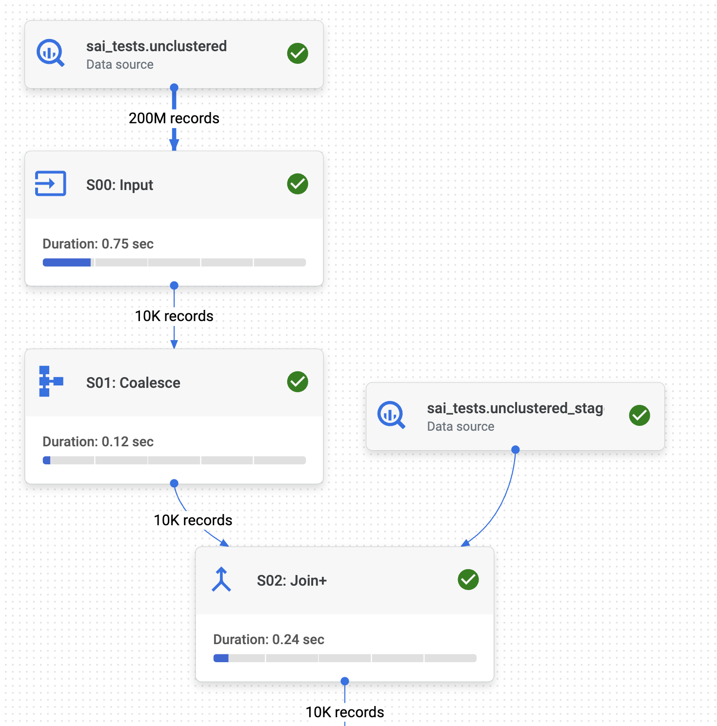
Now let us analyze important step of the execution graph:
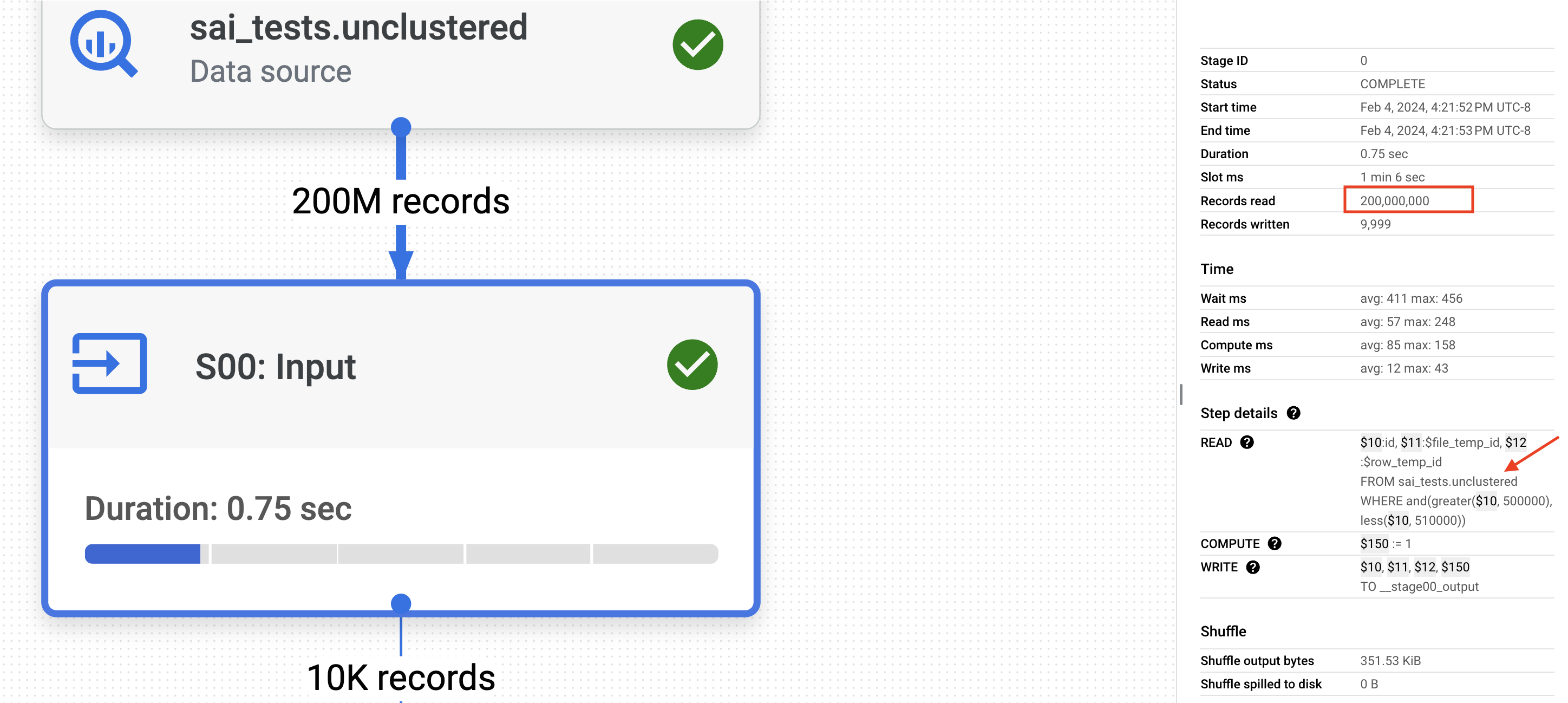
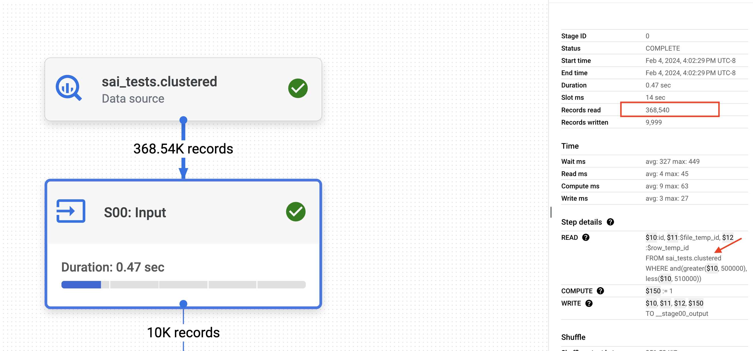
In the first step (S00), BigQuery infers the join across both tables and pushes the
idfilter to the final table. Despite pushing the filter down to the final table, BigQuery still reads all 200 million records to retrieve the approximately 10K filtered records. This is due to the absence of clustering on the 'id' column in the final table.Now, let us analyze the JOIN (S02). As a part of the JOIN, BigQuery scans the entire 10 million records in the staging table, even though there is a WHERE clause on the
idthat filters approximately 10K records. This is due to the absence of clustering on theidcolumn in the staging table.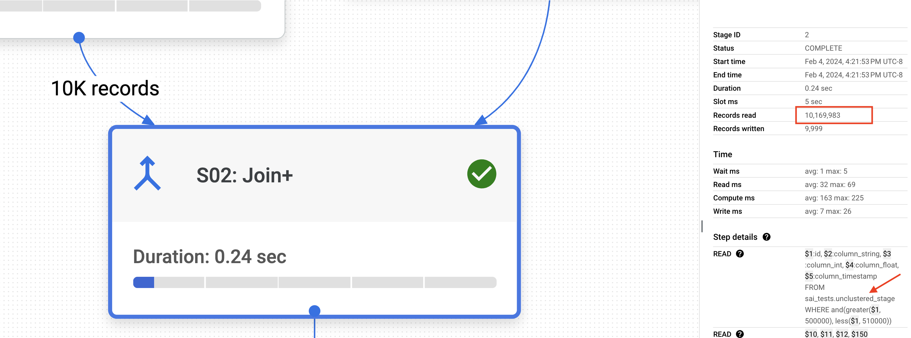
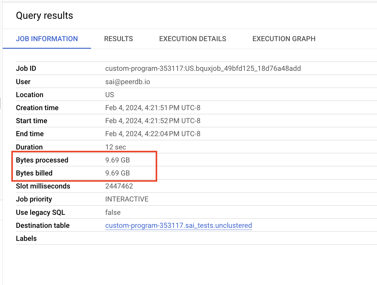
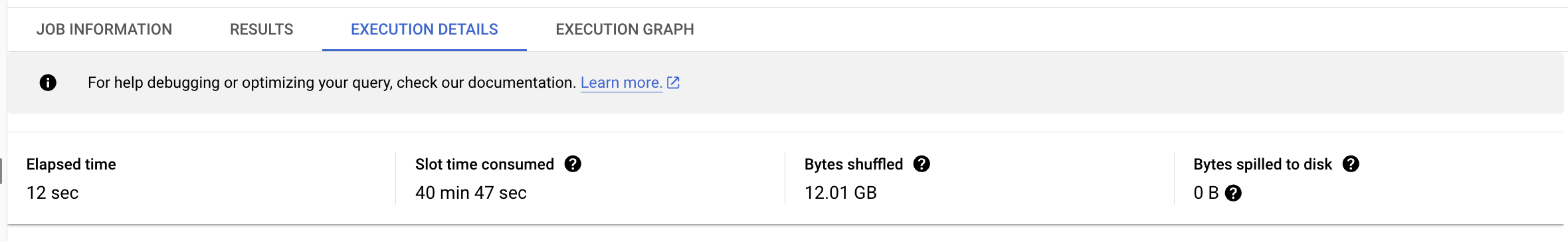
If you observe, lack of CLUSTERING made BigQuery generate suboptimal plan processing 9.69GB of data costing 4.7 cents.
Analyzing the MERGE command on the Unclustered tables
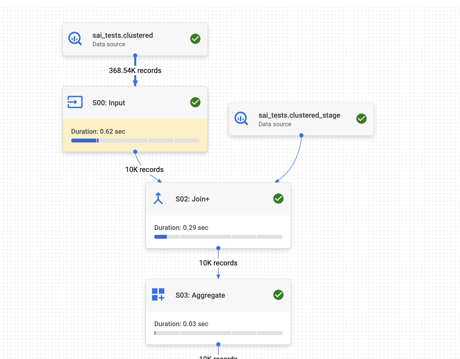
Below is the execution graph of the MERGE command on the clustered tables:
Now let us analyze each step of the execution graph:
First, BigQuery infers the join across both tables and pushes the
idfilter to the final table. Since the final table is CLUSTERED on theidcolumn, BigQuery leverages this clustering to efficiently retrieve approximately 368K records out of the 200 million records in the final table.Now, let's analyze the JOIN (S02). As part of the JOIN, BigQuery utilizes the CLUSTERED
idto read only 362K records from the staging table, which contains 10 million records.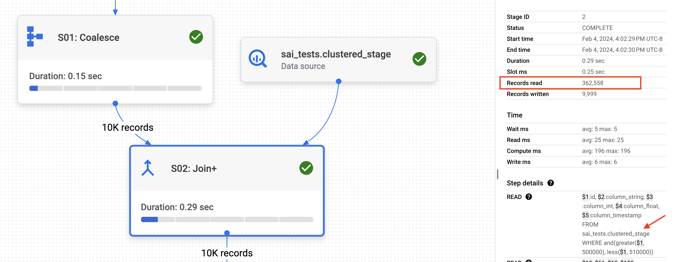
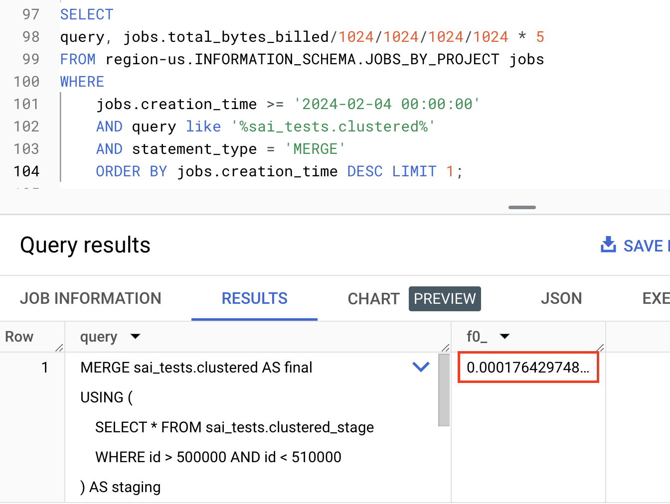
If you observe BigQuery optimally filtered data across both the staging and final table using the
CLUSTER(index) on id processing only ~37MB of data costing 0.017 cents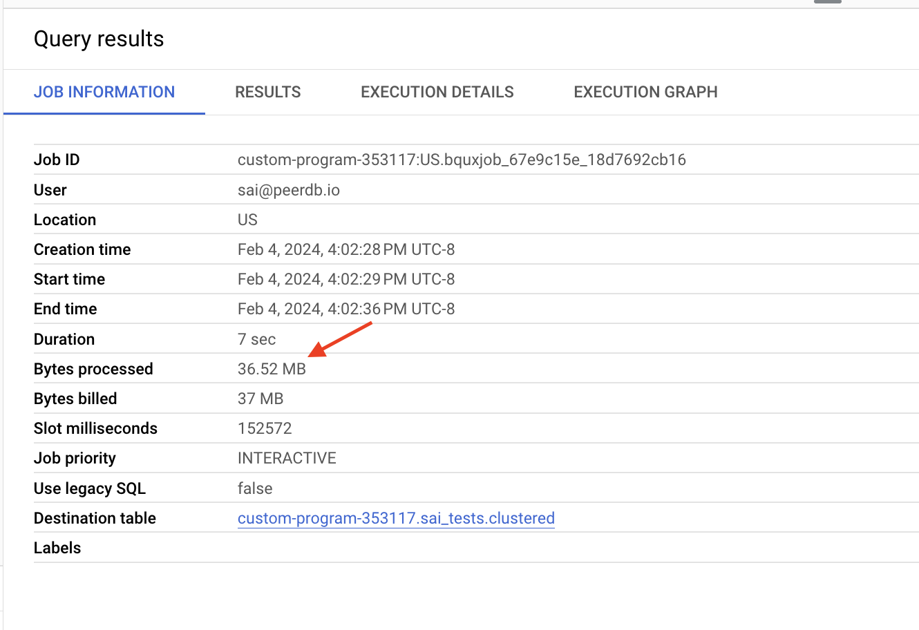

Results: Unclustered vs Clustered Tables
| Unclustered | Clustered | Difference | |
| Bytes Processed | 9.69GB | 37MB | ~260X |
| Slot time | 40.5min | 2.5min | ~20x |
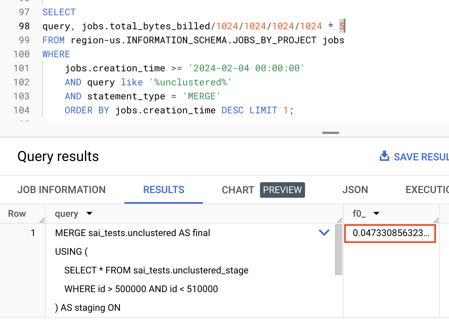
| Costs | 4.7 cents | 0.017 cents | ~268X |
The amount of bytes processed by the MERGE on the clustered set of tables is 260 times lower than the unclustered group.
Slot time is 20 times lower on clustered tables compared to unclustered tables.
Costs ($$) are 268 times lower for MERGE on clustered tables compared to unclustered tables.
This is the impact a simple CLUSTER can have on compute costs for BigQuery. Based on the MERGE commands that you use, observe the join columns and columns in the WHERE clause, and intelligently CLUSTER tables on those columns. This can signficantly reduce costs. With a similar approach.
Auto Clustering and Partitioning in PeerDB
We at PeerDB are building a fast and cost-effective way to replicate data from Postgres to Data Warehouses and Queues. Aligned with the above blog post, we automatically cluster and partition the raw and the final tables on BigQuery. The raw table is cluster based on 2 columns that have WHERE clause filters and partition based on timestamp. The final table is clustered based on the primary key. We've seen significant cost reduction (2x-10x) for our customers with this optimization.
References
Hope you enjoyed reading the blog, here are a few references that you might find interesting:
Shopify reduced their BigQuery spend from ~$1,000,000 to ~$1000.
Visit PeerDB's GitHub repository to Get Started.