Moving a Billion Postgres Rows on a $100 Budget

Inspired by the 1BR Challenge, I wanted to see how much it would cost to transfer 1 billion rows from Postgres to Snowflake. Moving 1 billion rows is no easy task. The process involves not just the transfer of data but ensuring its integrity, error recovery and consistency post-migration.
Central to this task is the selection of tools and techniques. We will discuss the use of open-source tools, customized scripts, ways to read data from Postgres, and Snowflake’s data loading capabilities. Key aspects like parallel processing, efficiently reading Postgres’ WAL, data compression and incremental batch loading on Snowflake will be highlighted.
I will list and discuss some of the optimizations that are implemented to minimize compute, network, and warehouse costs. Additionally, I will highlight some of the trade-offs made as part of this process. Given that most of the approaches covered in this blog stem from my explorations at PeerDB aimed at enhancing our product – The task was accomplished primarily through PeerDB.
I want to make it clear that there are some feature gaps in comparison to a mature system, and it might not be practical for all use cases. However, it does handle the most common use cases effectively while significantly reducing costs. I also want to caveat that there might be some ways in which the estimations may be off and I’d be happy to adjust based on feedback.
Setup
Initial data load: We will consider that there are 300M rows already in the table at the start of the task, and our system should handle the initial load of all the rows.
Inserts, Updates and Deletes (Change Data Capture): The rest of the 700M rows will be a combination of inserts, updates and deletes. Including support for toast columns.
- 1024 rows changed per second for ~8 days.
Recoverability: We will reboot the system every 30 mins to ensure that it's robust and can recover from disasters.
Now let us walk through an engineering design that optimally handles the above workload with the objective of minimizing costs and improving performance, one step at a time.
Initial Load from Postgres to Snowflake
Let’s start with the first operation any data sync job has to do: load the initial set of data from the source to destination. There are a few challenges that come with this:
How to efficiently retrieve large amounts of data from Postgres?
How to process the data in a way where we have minimal cost foot-print?
How to efficiently load this data to Snowflake?
Optimal Data retrieval from Postgres
Reading a table sequentially from Postgres is slow. It would take a long time to read 300M rows from Postgres. To make this process more efficient, we have to parallelize. We've got a clever way to quickly read parts of a table in Postgres using something called the TID Scan, which is a bit of a hidden gem. Basically, it lets us pick out specific chunks of data as stored on disk, identified by their Tuple IDs (CTIDs), which look like (page, tuple). This optimizes IO utilization and is super handy for reading big tables efficiently.
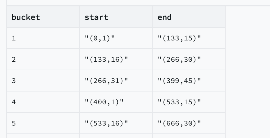
Here's how we do it: we divide the table into partitions based on the pages of the database, and each partition gets its own scan task. Each task handles about 500K rows. So, we partition the table into CTID ranges, with each partition having ~500K rows, and we process each partition parallelly (16 partitions at a time).
SELECT count(*) FROM public.challenge_1br; -- find the count

-- num_partitions = (count // rows_per_partition)

SELECT bucket, MIN(ctid) AS start, MAX(ctid) AS end
FROM (
    SELECT NTILE(1000) OVER (ORDER BY ctid) AS bucket, ctid
  FROM public.challenge_1br
) subquery
GROUP BY bucket ORDER BY start;
Data in Transit
It is important to process the data in a way where we don’t overload the system. As we are operating under budget constraints, we need to use techniques that use the hardware effectively. We are going to be using the “your dataset fits in RAM'' paradigm of systems design. 300M rows for initial load does sound like a lot, but let's see how we can make it fit in our RAM. We need to process the data to ensure data-types are mapped correctly to the destination. We are going to convert the query results to Avro for faster loading into warehouses, and also for its logical type support.
How big is the data?
Let us take a little detour to explore how big the data is. This is a good chance to look at some real world examples to estimate things. Based on interacting with a lot of production customers, and talking to some experts, it’s safe to say that on an average we see ~15 columns per table. In our table, let’s say each row is ~512 bytes.
# for initial load
num_rows = 300_000_000
bytes_per_row = 512
total_num_bytes = num_rows * bytes_per_row
total_size_gb = total_num_bytes / 1_000_000_000
# total initial load size 153.6 GB

# memory required during initial load

num_rows_per_partition = 500_000
mb_per_partition = num_rows_per_partition * bytes_per_row / 1_000_000 # 256 MB
num_partitions_in_parallel = 16
required_memory = num_partitions_in_parallel * mb_per_partition # 4096 MB
Required Memory
Based on the above napkin math, we can see that with 4GB of RAM we should be able to do the initial load. We will allocate 8GB of RAM to account for other components.
Efficiently loading data into Snowflake
As mentioned earlier we are going to store the query results into Avro on-disk. We are further going to compress the Avro files using zstd to further reduce the disk footprint and also to save on network costs. We will take a slight deviation from the topic to talk about Bandwidth costs.
Bandwidth costs: They can break the bank!
Let's look at the network costs, you can see the variance in numbers.
| Cost per 10GB (egress) | AWS | GCP | Azure |
| Within same AZ | Free | Free | Free |
| Within same region (different AZ) | $0.1 | $0.1 | $0.1 |
| Across Regions | $0.1 - $0.2 (Depends on Destination) | $0.2 - $1.4 (Depends on source+destination) | $0.2 - $1.6 (Depends on region + +intra/inter continental) |
| To Internet | $0.9 - $0.5 (10TB - 150TB) | $0.8 - $2.3 (Premium tier - Depends on Source+Destination) | $1.81 - $0.5 (MS Premium NW - Depends on source + usage) |
It’s interesting to see the variance in the costs, so it’s best to have Postgres, our System and Snowflake in the same cloud provider and the same region. Let’s now calculate the networks costs needed for this workload.
Calculating Network Costs
Another thing to be wary of is the Warehouse configuration.
bytes_per_row = 512
num_rows = 1_000_000_000
total_data_size = 512GB
compressed_data_size_GB = 256 #avro+zstd gives atleast 2x compression
bandwidth_cost_per_10GB = $0.1

# total nework costs
# data_size_GB * bandwidth_cost_per_10GB / 10
network_costs_egress_from_postgres = $5
# compressed_data_size_GB * bandwidth_cost_per_10GB / 10
network_costs_egress_from_system_to_snowflake = $2.56

network_costs = $7.56
Snowflake Warehouse Configuration
In many organizations, a significant portion of Snowflake expenses comes from compute usage, particularly when warehouses run idle between tasks. Snowflake's compute costs are accrued based on warehouse operational time, starting from activation to suspension. Often, idle warehouse time can contribute to 10%-25% of the total Snowflake compute costs. The Baselit team wrote an excellent blog about it: read more about it here.
The two things we will be doing is to set AUTO_SUSPEND to be 60 seconds, a warehouse idles for up to a minute after the last query before pausing, and make sure that we keep the warehouse active for the least amount of time. This is the default configuration you get if you follow the PeerDB Snowflake setup guide.
Inserts, Updates and Deletes
The next challenge for us after the initial load would be to read the change data from Postgres and replaying that to Snowflake. We are going to be doing that using Postgres’ Logical Replication. At the start of the replication, we will create a replication slot and use pgoutput plugin. This is the recommended way to read changes from the slot. Once we read the changes from the slot, we will batch them and then load them to Snowflake.
As we discussed earlier, it is important to keep the Snowflake warehouse idle for as long as we can, and batching helps with that. We store records in batches of 1M to Avro like before, and load them to an internal stage in Snowflake. Once the data is loaded into the stage, we will MERGE the records from the stage into the destination table. This way most of the heavy-lifting of the resolution is left to the warehouse and it simplifies our system.
Tools
At PeerDB, we are building a specialized data-movement tool for Postgres with laser focus on Postgres to Data Warehouse replication. Most of the above optimizations incl. parallel initial load, reducing Data Warehouse costs, native data-type mapping, support of TOAST columns, fault-tolerance and auto recovery etc. are already baked into the product. PeerDB is also Free and Open. So we chose PeerDB to implement the above workload.
Hardware
Now that we have landed on 8GB RAM, let us move onto picking the instance type.
Since ARM uses lower energy compared to x64 (due to being RISC), they are around 25% cheaper as compared to x64 machines. The tradeoff here is that x64 machines run at around 2.9GHz with a 3.5GHz Turbo (M6i instances) as compared to ARM machines at about 2.5GHz (Graviton2 - M6g) but M6i instances are about 30% more expensive as compared to M6g instances.
Effective cost is $0.0409/GHz for x64 vs $0.03616/GHz for ARM, so cost is about 13% more per GHz on x64 But cost per GHz is not the determining factor for reading in a single thread from Postres during CDC as replication slots can be read from a single process at once.
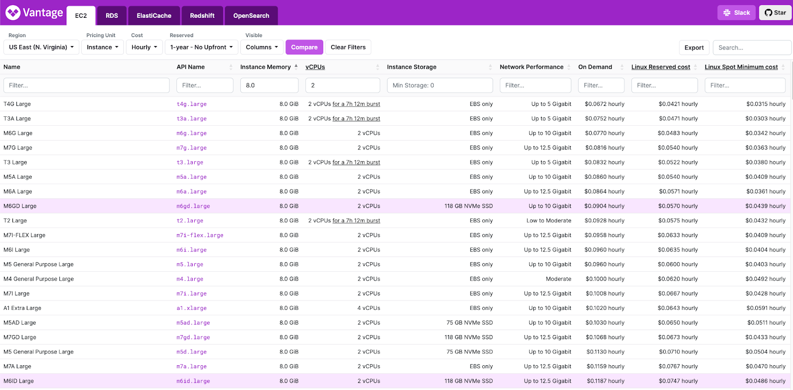
For this current experiment, I went with m6gd.large as it offers a good balance of speed and disk.
Optional read: In this blog we will use AWS for our analysis. However, here are some other learnings we had on this topic. OVH Cloud currently does not support ARM Instances and has a similar $0.118/hour c2-7 instance (in limited regions) which has a very low network speed (250MBps) with 50GB of SSD. Hetzner has a CCX13 $0.0292/hour instance (including a 118GB SSD) but no dedicated ARM instances.
Conclusion
One question that I'm often posed with: “Is this practical?”. Yes, one machine can die, but systems where there is only one machine have a remarkable amount of uptime, especially when the state is stored in a durable way.
Back to the topic at hand. If we look at the total cost of the system we built (assuming us-west-2 as the region. Over a month time this is the breakdown:
| Cost Category | Cost | Comment |
| Hardware | $65.992 / month | AWS m6gd.large (2 vcpus, 8 GB RAM) |
| Comes with 118 GB NVMe which is great! | ||
| Network | $7.56 | AWS network transfer same region 500 GB (with compression) |
| Warehouse | N/A | These are common across various vendors |
| Total | $73.552 | Hardware Costs + Network costs = $65.992 + $7.56 = $73.552 (Within $100 budget) |
If we were to look at various ETL tools and how much they charge for moving 1 billion rows, this is what it comes out to:
| Vendor | Cost per 1 billion records |
| Fivetran | $23,157.89 |
| Airbyte | $11,760.00 |
| Stitch Data | $4,166.67 |
| Above Approach (using PeerDB OSS) | $73.552 |
I am part of a company building a software for moving data specifically from Postgres to Data warehouses. It's my job to figure out how to provide the best experience to our customers. Doing this project forced me to figure out a way to provide the best bang for buck, and to include a lot of the explored features into PeerDB. I hope it conveys some appreciation for what modern hardware is capable of, and how much you can get out of it.